WHAT'S YOUR INTERPRETATION?
 Scatterplots
can be very useful in helping to identify associations between
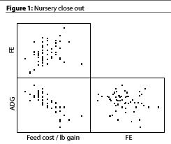
and among several variables. Looking at the data depicted in Figure
1 (on the cover) in relation to feed cost per lb of gain, there
appear to be two important associations: average daily gain (ADG)
and feed efficiency (FE), both of which appear to have strong
associations with feed cost per lb of gain.
These multiple scatter plots were generated by the programmed SPC/PI version 2.46 (Qualitran Professional Services, Inc.), which can generate a graph including up to seven different variables. In this example, just two variables were used for simplicity. The option to use multiple variables can be a very powerful way to quickly scan the data for possible associations. One can then go on to perform the appropriate statistical test.
 Let's assume our question is: how
does one change the feed cost per lb of gain when looking at ADG
and FE? Which one of these variables would have the greatest impact
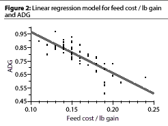
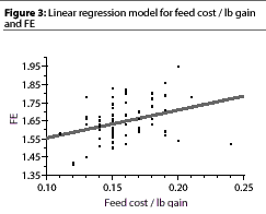
in this system? After generating a scatterplot like those shown
in Figures 2 and 3, the next step is to run a regression on these
two variables to see whether there is any significance and how
much of the variation in the data can be explained.
When evaluating the statistical output of the data shown in Figure 2, the ADG linear regression model had a P value <0.0001 and an R2 of .615. This means that 61.5% of the variation in feed cost per lb of gain can be explained by ADG. So if we can increase ADG we should see a lower feed cost per lb of gain.
 The linear regression results of
the data shown in the FE model (Figure 3) had a P <.
001 and an R2 of .113. This tells us there is a significant
association between FE and feed cost per lb of gain. This association
is expected. What is not expected is that in this data set, FE
explains only 11.3 % of the variation in feed cost per lb of gain.
In the example data set shown here, there were no significant associations between ADG and FE.
Both FE and ADG were significant variables in feed cost per lb of gain. In this system, the most predictable change in feed cost per lb of gain would come from increasing ADG in the system. This could possibly mean that the average FE is closer to where it is expected to be and if ADG can be increased, this would make a more significant change in feed cost per lb of gain. Feed cost per lb of gain can significantly influence overall cost per lb of gain; however, this was not evaluated in this example model. Using scatterplots to look for an association is very valuable but must be tied in with other statistical tests. The data shown in this example are specific to this farm and may not necessarily generalize to all farms. The unique differences among farms make it very important to analyze data for each specific farm. This way the data can give us more information and help us to better predict expected changes.
--Dr. Paul Yeske
Swine Vet Center PA, St. Peter, Minnesota
